Implementing a Time Series Forecast in Python
To practice the implementation of a time series and turn all the above concepts into code, we will be working on the same daily climate change dataset that was previously introduced in this chapter. The aim of this forecasting is to predict how the measures of mean air pressure, wind speed, etc. will line up in the future. (We will be forecasting the data for six future time periods)
Before we begin there are a few concepts we should revisit, to understand the working of time series better. One of the concepts is the
Ad-Fuller Test or augmented Dickey–Fuller test (ADF) that tests the null hypothesis that a unit root is present in the data that represents the time series. The ADF statistic that is part of this test is always a negative number. The theory is, that, the more negative this statistic gets, the stronger is the rejection of the null hypothesis. Another concept we will drive through is
VAR (Vector Auto Regressions). The VAR statistical model is used to study the relationship of numerous dependent quantities present in the time series data that have the tendency to change with time periods. The multivariate model of fitting, allows for using the lag over time variable and forms its predictions based on the input lag values.
# Importing the basic preprocessing packages
import numpy as np
import matplotlib.pyplot as plt
import pandas as pd
# The series module from Pandas will help in creating a time series
from pandas import Series,DataFrame
%matplotlib inline
# Statsmodel and Adfuller will help in testing the stationarity of the time series
import statsmodels
from statsmodels.tsa.stattools import adfuller

time_series_train = pd.read_csv('DailyDelhiClimateTrain.csv', parse_dates=True)
time_series_train["date"] = pd.to_datetime(time_series_train["date"])
time_series_train.date.freq ="D"
time_series_train.set_index("date", inplace=True)
time_series_train.columns


>>> Index(['meantemp', 'humidity', 'wind_speed', 'meanpressure'], dtype='object')


# Decomposing the time series with Statsmodels Decompose Method
from statsmodels.tsa.seasonal import seasonal_decompose
sd_1 = seasonal_decompose(time_series_train["meantemp"])
sd_2 = seasonal_decompose(time_series_train["humidity"])
sd_3 = seasonal_decompose(time_series_train["wind_speed"])
sd_4 = seasonal_decompose(time_series_train["meanpressure"])
sd_1.plot()
sd_2.plot()
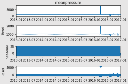
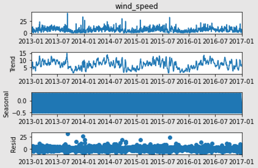
sd_3.plot()
sd_4.plot()
>>>

.png.aspx;)
.png.aspx;)

# From the above graph’s observations, it looks like everything other than meanpressure is already stationary

# To re-confirm stationarity, we will run all columns through the ad-fuller test
adfuller(time_series_train["meantemp"])


>>>
(-2.021069055920669,
 0.277412137230162,
 10,
 1451,
 {'1%': -3.4348647527922824,
  '5%': -2.863533960720434,
  '10%': -2.567831568508802},
 5423.895746470953)


adfuller(time_series_train["humidity"])


>>>
(-3.6755769191633343,
 0.004470100478130829,
 15,
 1446,
 {'1%': -3.434880391815318,
  '5%': -2.8635408625359315,
  '10%': -2.5678352438452814},
 9961.530007876658)


adfuller(time_series_train["wind_speed"])


>>>
(-3.838096756685103,
 0.0025407221531464205,
 24,
 1437,
 {'1%': -3.434908816804013,
  '5%': -2.863553406963303,
  '10%': -2.5678419239852994},
 8107.698049704068)


adfuller(time_series_train["meanpressure"])


(-38.0785900255616,
 0.0,
 0,
 1461,
 {'1%': -3.434833796443757,
  '5%': -2.8635202989550756,
  '10%': -2.567824293398847},
 19034.033348261542)


# Consolidate the ad-fuller tests to test from static data
temp_var = time_series_train.columns
print('significance level : 0.05')
for var in temp_var:
    ad_full = adfuller(time_series_train[var])
    print(f'For {var}')
    print(f'Test static {ad_full[1]}',end='\n \n')


>>>
significance level : 0.05
For meantemp
Test static 0.277412137230162
For humidity
Test static 0.004470100478130829
For wind_speed
Test static 0.0025407221531464205
For meanpressure
Test static 0.0


# With the ad-fuller test, we can now conclude that all data is stationary since static tests are below significance levels. This also rejects the hypothesis that meanpressure was non-static.

# Let us now move towards training and validating the prediction model

from statsmodels.tsa.vector_ar.var_model import VAR
train_model = VAR(time_series_train)
fit_model = train_model.fit(6)

# AIC is lower for lag_order 6. Hence, we can assume the lag_order of 6.
fix_train_test = time_series_train.dropna()
order_lag_a = fit_model.k_ar
X = fix_train_test[:-order_lag_a]
Y = fix_train_test[-order_lag_a:]

# Model Validation
validate_y = X.values[-order_lag_a:]
forcast_val = fit_model.forecast(validate_y,steps=order_lag_a)
train_forecast = DataFrame(forcast_val,index=time_series_train.index[-order_lag_a:],columns=Y.columns)
train_forecast


>>>
 date       meantemp	humidity	wind_speed	meanpressure
2016-12-27	17.348792	70.642850	7.421823	1114.035254
2016-12-28	17.726869	68.599848	6.255075	1010.853957
2016-12-29	17.496228	70.909252	6.333213	992.402101
2016-12-30	17.648930	72.704921	5.795082	1004.788372
2016-12-31	17.642094	73.481324	5.946337	1031.434268
2017-01-01	17.884142	72.291600	5.717422	1026.203648


# Check performance of the predictions’ model
from sklearn.metrics import mean_absolute_error
for i in time_series_train.columns:
    print(f'MAE of {i} is {mean_absolute_error(Y[[i]],train_forecast[[i]])}')


>>> MAE of meantemp is 2.8822831810975056
>>> MAE of humidity is 13.130988743454763
>>> MAE of wind_speed is 1.920218001710155
>>> MAE of meanpressure is 27.450580288019903


# Humidity and Meanpressure are showing higher errors of forecast. We could assume that certain external factors are causing this.
# This model, therefore, forecasts wind speed and mean temperature accurately with less than 5% error
# Let us now implement this on the test data and forecast for the next 6 future periods of time

test_forecast = pd.read_csv('DailyDelhiClimateTest.csv',parse_dates=['date'])
period_range = pd.date_range('2017-01-05',periods=6)
order_lag_b = fit_model.k_ar
X1,Y1 = test_forecast[1:-order_lag_b],test_forecast[-order_lag_b:]
input_val = Y1.values[-order_lag_b:]
data_forecast = fit_model.forecast(input_val,steps=order_lag_b)
df_forecast = DataFrame(data_forecast,columns=X1.columns,index=period_range)
df_forecast


>>>

  date       meantemp	humidity	wind_speed	meanpressure
2017-01-05	32.268428	29.294430	9.273689	1028.807335
2017-01-06	32.404384	33.362166	8.264082	996.529808
2017-01-07	32.420385	36.232933	8.283705	982.572684
2017-01-08	32.148770	38.216824	8.446112	997.883636
2017-01-09	32.057660	38.568787	8.467237	1020.024659
2017-01-10	32.083931	38.433189	8.478052	1037.946455


# Plotting the test data with auto correlation

from statsmodels.graphics.tsaplots import plot_acf

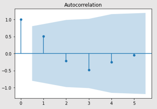
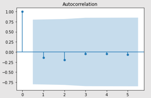
# The next 6 periods of mean temperature (graph 1) and wind_speed (graph 2)
plot_acf(df_forecast["meantemp"])
plot_acf(df_forecast["wind_speed"])


# With this we conclude the Time Series Forecasting of Daily Climate Data from a city.
Now that we have understood how to implement a Time Series forecast for data that changes over time, let us understand a few key concepts that play an important role in making the prediction model accurate.
Understanding Autocorrelation and Partial Correlation
Lags in Time Series: Lag, as a general English term refers to slower response time, often called latency. In a time-series forecast or analysis a lag in the range of 1 to 8 is considered appropriate for quarterly timed data. For a monthly spaced time-series, lags of 6, 12 or 24 are considered appropriate. To understand lags better, let us take this scenario. For a discrete set of values that belong to a time series, for lag 1, the comparison of this time series will be made with the same time series at a period before the current one. In other words, the time series is shifted to one time period in the past.
Autocorrelation: The correlation between the series and its lags is called autocorrelation. Like correlation that measures the magnitude to which a linear relationship is associated between two variables, autocorrelation does the same between lagged values of a time series. If the series is considerably autocorrelated, it means that the impact of lags on forecasting the time series is high. In more general terms, a correlation factor of 1 (Lag = 1) conveys the correlation between values that are one period apart from each other. Likewise, lag ‘k’ autocorrelation shows the association amongst values that are ‘k’ time periods separately from each other.
Partial Autocorrelation: The purpose of partial autocorrelation is also like autocorrelation as it conveys the information about the relationship between a variable and its lag. But partial autocorrelation only delivers details about pure association between the lag and disregards correlations that occur from intermediate lags.
Granger Causality Test for forecasting time series
The Granger causality test helps in understanding the behavior of a time series by analyzing a similar time series. The test assumes that if an event X causes the occurrence of another event Y, then the future predictions of Y based on the preceding values of Y and X combined, should outdo the forecasting of Y that is based on Y individually. Therefore, something to note here is that Granger Causality should ideally not be used in conditions where a lag of the event Y is causing Y.
The statsmodel package with PyPi implements Granger Causality test. The method accepts a 2-dimensional array with two columns as its main argument. The first column contains the values, and the predictor (X) is contained in the second column. The null hypothesis here is that the series that belongs to the second column, does not cause the occurrence of the series that is part of the first column. The null hypothesis is rejected if the P-values are lesser than the pre-defined significance level of 0.05. This also concludes that the lag of X is useful. The second argument “maxlag” allows you to input the maximum number of lags of Y that need to be included in the test
Let us know take this knowledge and implement the Granger Causality test for the Daily Climate dataset.
# Import Granger Causality module from the statsmodels package and use the Chi-Squared test metric
from statsmodels.tsa.stattools import grangercausalitytests
test_var = time_series.columns
lag_max = 12
test_type = 'ssr_chi2test'

causal_val = DataFrame(np.zeros((len(test_var),len(test_var))),columns=test_var,index=test_var)
for a in test_var:
    for b in test_var:
        c = grangercausalitytests ( time_series [ [b,a] ], maxlag = lag_max, verbose = False)
        pred_val = [round ( c [ i +1 ] [0] [test_type] [1], 5 ) for i in range (lag_max) ]
        min_value = np.min (pred_val)
        causal_val.loc[b,a] = min_value
causal_val


>>>

			   humidity       wind_speed   mean        pressure
meantemp	   1.00000	      0.00382	   0.00054     0.22012
humidity	   0.00000	      1.00000	   0.13319     0.15053
wind_speed	   0.00000	      0.00000	   1.00000     0.52294
meanpressure	0.00633	      0.43641	   0.04252     1.00000


# The results of the Granger Causality justify that the features are closely dependent on each other
We now conclude the study of Time Series Forecasting. Although, Time Series is a vast topic and includes various other singularities that were not discussed in this chapter, this should be considered a start for this area of study. Analysis starts with studying time series data, understanding stationarity, testing it for seasonality, building models of prediction and finally moving on to the forecasting of time.
Coming Up Next
With Time Series Forecasting, we have now completed the basics of Machine Learning. Classification and Clustering machine learning algorithms help in predicting values that are part of a larger input group. Regression also helps in categorizing and predicting the independent variables from the dependent ones. Along with analysis of time series data, we can forecast values and findings at a later point of time along the future based on historical data. In the coming section we will use the knowledge of these machine learning algorithms to build a case study project.
- Revisiting data preprocessing and cleaning
- Traversing through a machine learning problem
- Solving a real-world problem using machine learning