Introduction
Time Series is a sequence of data that is present in intervals of time. These intervals can be hourly, daily, weekly, or any quantifiable repetitive duration of time. A sequence of these observations made over regular time intervals is called time series. Forecasting time series deals with predicting the next cycle or observation of events that would occur in a future-referenced time frame. We will walk through forecasting Time Series in this chapter.
Understanding the flow of Time Series Forecasting
/5-1.png.aspx;)
Sequence Analysis and its Importance
In the present era, every business is using Machine Learning to understand the behavior of their customers and forecast sales and acquisitions. Besides, time series forecasting has massive commercial and consumer marketing importance because things that are important to a business, like demand, sales quotes, number of people visiting a website, stock price predictions, etc. are essentially time series data where forecasting helps. We start the analysis by understanding numerous aspects of the nature of data and its dependency on time.
Panel Data: Panel is a time-based dataset that in addition to sequential data also contains one or more linked variables that are quantified for same periods of time. These dependent variables help in providing valuable insights for predicting the value of ‘Y’. One way to understand whether a dataset is time series or panel, is to understand if the time column is the only part of data that is affecting the outcome of the prediction.
Time series analysis is applicable to real-valued numerical data, continuous data, discrete numerical data, as well as discrete symbolic data (that is, series of characters, such as letters and words of a language).
Important Python packages and Libraries for Time Series Analysis
To analyze time series and to build prediction models on time series, let’s take a look at some important libraries and methods.
- Stattools: It is a PyPi package that implements Statistical learning and several algorithms for calculating inference in data. Supported in Python versions 3.6 and above.
- Pandas Dataframe Resample: Resampling is a technique used for changing the frequency of time series observations. Within pandas' data frames, the resample method makes this frequency conversion convenient. Pre-conditions required are, that the object must have datetime data type formats (datetime, datetimeindex, periodindex, timedeltaindex, etc.). There exist two resampling types, namely:
- Upsampling: The frequency of sample data is increased. For instance, changing a minute-based frequency to seconds.
- Downsampling: The vice-versa of unsampling. Example, changing a day-based frequency to months.
- pmdarima: Originally called pyramid-arima, pmdarima is a statistical library that aids in filling data voids in Python's time series. It contains a collection of statistical tests for checking stationarity and seasonality. Features such as differencing of time series and inverse differencing are also included.
Performing some Statistical Functionalities on Time Series data:
# Importing the basic preprocessing packages
import numpy as np
import matplotlib.pyplot as plt
import pandas as pd
# The series module from Pandas will help in creating a time series
from pandas import Series,DataFrame
import seaborn as sns
%matplotlib inline

# About the Data Set (Location: https://www.kaggle.com/sumanthvrao/daily-climate-time-series-data)
# To forecast the daily climate of a city in India
time_series = pd.read_csv('DailyDelhiClimateTrain.csv', parse_dates=['date'], index_col='date')
time_series.head()


>>>
	meantemp	humidity	wind_speed	meanpressure
date
2013-01-01	10.000000	84.500000	0.000000	1015.666667
2013-01-02	7.400000	92.000000	2.980000	1017.800000
2013-01-03	7.166667	87.000000	4.633333	1018.666667
2013-01-04	8.666667	71.333333	1.233333	1017.166667
2013-01-05	6.000000	86.833333	3.700000	1016.500000


# Below are a few statistical methods on time series that will help in understanding the data patterns
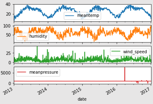
# Plotting all the individual columns to observe the pattern of data in each column
time_series.plot(subplots=True)


>>>
array([, ,
       , ],
      dtype=object)

# Calculating the mean, maximum values, and minimum of all individual columns of the dataset
time_series.mean()


>>>
meantemp          25.495521
humidity          60.771702
wind_speed         6.802209
meanpressure    1011.104548
dtype: float64


time_series.max()


>>>
meantemp          38.714286
humidity         100.000000
wind_speed        42.220000
meanpressure    7679.333333
dtype: float64


time_series.min()


>>>
meantemp         6.000000
humidity        13.428571
wind_speed       0.000000
meanpressure    -3.041667
dtype: float64


# The describe() method gives information like count, mean, deviations and quartiles of all columns
time_series.describe()


>>>
meantemp	humidity	wind_speed	meanpressure
count	1462.000000	1462.000000	1462.000000	1462.000000
mean	25.495521	60.771702	6.802209	1011.104548
std	7.348103	16.769652	4.561602	180.231668
min	6.000000	13.428571	0.000000	-3.041667
25%	18.857143	50.375000	3.475000	1001.580357
50%	27.714286	62.625000	6.221667	1008.563492
75%	31.305804	72.218750	9.238235	1014.944901
max	38.714286	100.000000	42.220000	7679.333333


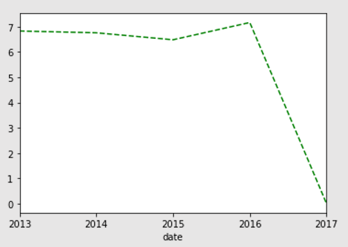
# Resampling the dataset using the Mean() resample method
timeseries_mm = time_series['wind_speed'].resample("A").mean()
timeseries_mm.plot(style='g--')
plt.show()

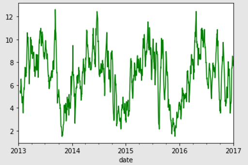
# Calculating the rolling mean with a 14-bracket window between time intervals
time_series['wind_speed'].rolling(window=14, center=False).mean().plot(style='-g')
plt.show()
>>>

# In the coming sections we will implement time series forecasting on the same dataset
Stationary and Non-Stationary Time Series
Stationarity is considered a feature in every time series. In case of a stationery series, the values of the time series are not a function of time. Which means that measure like mean, variance, and autocorrelation of current values with past values, are all constant over time. A stationary time series is also not affected by seasonal changes. Almost every time series can be made stationary by applying appropriate transformations.
Making a Time Series Stationary
Time Series data can be made stationary using any of the following mentioned procedures:
- Differencing the series once or more: The concept of differencing states that subtracting a series value in the current time by a value of the same series in a previous unit of time will make it stationary. Meaning, subtracting the next value by the current value is differencing.
- For example, consider the following series: [1, 5, 2, 12, 20]. First differencing gives: [5-1, 2-5, 12-2, 20-12] = [4, -3, 10, 8]. Differencing it the second time gives: [-3-4, -10-3, 8-10] = [-7, -13, -2]
- Taking the Log of the existing Time Series
- Taking the N-th root of the current series.
- Combining one or more of the above techniques.
Why is a Stationary Time Series important?
A stationary time series is comparitively easy to forecast and is more reliable. The reason being, forecasting models are fundamentally linear regression algorithms that employ the lag(s) of these series data to form predictors.
We also know that linear regression algorithms work best in scenarios where the predictors (X) are not correlated among each other. Making a time series stationary removes all and any incessant autocorrelation between the predictors, hence, making the series better for regression to perform. Once the lag(s) or predictors of the series are independent, the forecasting is expected to give reliable predictions.
Seasonality and Dealing with Missing Values
Seasonality in time series data is the presence of variations that occur at specific intervals of time that is less than a year. These intervals can be hourly, monthly, weekly, or quarterly. Various considerations such as weather or climatic changes can cause seasonality. These patterns are always cyclic and occur in periodic patterns. Understanding seasonality is important for businesses whose work depends on these variations like stock markets, labor organizations, etc.
Seasonal Variations have several reasons of study and significance:
- The explanation of seasonal effects on a dataset provides a detailed understanding of the impact of seasonal changes on the data.
- Once a seasonal pattern in established, significant methodologies can be employed to eradicate it from the time series. This will help in studying the effects of other components of the dataset that are irregular in nature. De-seasonalizing is the concept of eliminating seasonality.
- Historical patterns of seasonality and regular variations help in forecasting future trends of the similar data. For example, prediction of climatic patterns.
Treating missing values within Time Series
It is very common to observe missing data in any dataset. Similarly, for data representing time series, it is possible to observe the series with missing dates or times. It could either mean that data for that time period was not captured, or that it was not available. It is always possible that data was captured and was zero. In which case, the false negative needs to be ignored. Also, an important point to note is, mean or median imputation is not a good practice to follow for time series data. Especially, if the time series is not exhibiting stationarity. A better and more sensible approach would be to fill the forward data with historical values of that time frame.
However, based on the study of the time series data and the landscape of the series, there are multiple approaches that can be tried to impute missing values. Some noteworthy and common techniques of imputing missing time series values are mentioned below:
- Backward Fill
- Linear Interpolation
- Quadratic interpolation
- Mean of nearest neighbors
- Mean of seasonal counterparts
It is also important to measure the performance of the time series after the new values have been introduced to the dataset. It is considered a good practice to use two or more ways of imputing the values and then calculating the accuracy of the model using methods like Root Mean Square (RMSE). This helps in deciding which imputation technique is best suited for the data.
This chapter continues in the following part two.