Regression
Through the journey into this course, we have established a connection between programming, mathematics, and statistical analysis to build a root for Machine Learning. In this chapter the focus will be on Regression in Machine Learning.
Regression based Analysis of Data
Regression analysis is a consortium of statistical techniques and procedures employed for the estimation of relationships between a singular dependent variable and one or more independent variables. Apart from classifying data, it is primarily also used to assess the potency of this relationship that exists between variables. It is also helpful for building forecasting of these variables in the future.

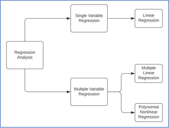
Image shows different types of Regression: Single Variable and Multivariate.
Non-collinearity: Independent variables in regression analysis are expected to show a minimum of correlation between each other. Also, in cases where independent variables show a very high correlation between each other, it becomes difficult to gauge the true relationships between them. Therefore, minimized collinearity is a mandatory condition for regression analysis to function.
SINGLE LINEAR REGRESSION
Expression:
Y = a + bX + epsilon, where
Y – Dependent variable
X – Independent (explanatory) variable
a – Intercept
b – Slope
epsilon – Residual (error)
MULTIVARIATE REGRESSION
Expression:
Y = a + bX1 + cX2 + dX3 + epsilon, where
Y – Dependent variable
X1, X2, X3 – Independent (explanatory) variables
a – Intercept
b, c, d – Slopes
epsilon – Residual (error)
Ensemble Modelling
Ensemble methods are a statistical technique that use multiple learning algorithms constituently to obtain a better predictive performance from the given input. Unlike the traditional statistical ensemble, machine learning models only work on a specific set of limited alternative models.
An example of understanding how Ensemble Modelling works, lets understand this scenario. If for instance, you are planning to purchase a car, would you choose the first car you learn about? Highly unlikely. You would want to research from varied sources to understand how different cars stack up against each other and then choose the best one for your needs. Ensemble training in machine learning algorithms does the exact same thing for classification and regression models.
Supervised Learning and Ensemble Importance
Supervised machine learning algorithms execute the tasks of moving through a predefined space of hypothesis to learn about the input and output to perform predictions. Ensemble combines multiple hypothesis together in the search of even better predictions.
Ensemble Techniques
Let us look at implementing ensemble techniques in machine learning algorithms.
- Max Voting: This method is generally used for classification problems, where multiple prediction scenarios are put against each other. Every individual model’s prediction is called a “vote”. The prediction value that is achieved from majority of the models, is chosen as the final output.
- Averaging: As the word suggests, in case of averaging problems, multiple predictions are made for a problem using different mechanisms. Finally, the average prediction of all these individual predictions is taken as the resultant value.
- Weighted Average: The extension of averaging technique is the weighted average technique. Every individual prediction model is assigned a weight of importance. For instance, if a research prediction is given by a professor who is experienced in research, his value will be given weightage over someone else’s who is new to the field.
Let us now look at the implementation of these Ensemble techniques in Python:
# Import scikit-learn library
import sklearn

# For instance, consider training a dataset using 3 distinct mechanisms – Decision Trees, KNN and Logistic Regression
model_one = sklearn.tree.DecisionTreeClassifier()
model_two = sklearn.neighbors.KNeighborsClassifier()
model_three = sklearn.linear_model.LogisticRegression()

# We fit these three models with the same training data
model_one.fit(x_train,y_train)
model_two.fit(x_train,y_train)
model_three.fit(x_train,y_train)

# Perform predictions on the same data, separately for the three algorithms
prediction_one = model_one.predict(x_test)
prediction_two = model_two.predict(x_test)
prediction_three = model_three.predict(x_test)

# One way to perform max voting algorithm is using the mode of all the predictions made through the three algorithms by iterating through every result
from statistics import mode
final_pred = np.array([])
for i in range(0,len(x_test)):
    final_pred = np.append(final_pred, mode([pred1[i], pred2[i], pred3[i]]))

# Sci-kit learn also gives a method VotingClassifier() to perform the Max Voting Ensemble Modelling
# sklearn.ensemble.VotingClassifier – It is a soft voting/majority rule classifier for unfitted estimators.
from sklearn.ensemble import VotingClassifier
model_one = LogisticRegression(random_state=2)
model_two = tree.DecisionTreeClassifier(random_state=2)

# estimators: it is the list of (str, estimator) tuples – when the fit method inside VotingClassifier() is called, clones of the original estimators are stored in the class attribute self.estimators_.
# voting{‘hard’, ‘soft’}, default=’hard’ – The voting variable takes in two arguments. Hard uses the predicted class labels for creating the majority rule, while soft uses the argmax of the predicted probabilities and creates labels for classes.
model_final = VotingClassifier(estimators=[('lr', model_one), ('dt', model_two)], voting='hard')
model_final.fit(x_train,y_train)
model_final.score(x_test,y_test)

# For performing Averaging in the Ensemble Model, we take the three predictions from separate models and calculate their average
final_prediction=(prediction_one + prediction_two + prediction_three) / 3

# By a similar approach, when calculating weighted averages, we give individual results a respective weight value and then take their average
final_prediction=(prediction_one * 0.3 + prediction_two * 0.4 + prediction_three * 0.7)
Ensemble Modelling is useful in regression analysis as it provides with the best-case scenario and combines results from multiple models to give the prediction.
Ensemble Representation:
/Image2-(1).png.aspx;?width=600&height=262)
Ensemble Techniques use a combination of multiple training algorithms and their respective predictions to form a suitable and best possible projection of the test data.
Regression in Machine Learning Algorithms
To build a regressor in Python, we will use the scikit-learn library that is used for Machine Learning. Here are some important functions and methods we need to understand before moving onto building a regressor.
- Single Regressor: Linear or Single regression works with two variables and attempts to work on a straight-line graph. It is used to establish a concrete relationship between two variables. The algorithm aims to draw a straight line that comes close to data points on both axes. It works by calculating the slope and intercept that eventually define the line function and minimize errors.
Using single regression in real-life: When predicting soil erosion, although external factors like temperature and animal traversal occur, they cause minimal damage to the soil. Predicting soil erosion has a direct relationship with rainfall. Therefore, the prediction of levels of soil erosion based on rainfall is an example of a single regression.
- Multivariable Regressor: Multivariable or Multivariate regression is an extension of single regression for use-cases when independent variables are more than one in number. These can be linear or non-linear. Multiple regressions are centered on an assumption that there exists a relationship between the dependent and independent variables of data.
Using multiple regression in real-life: In medicinal science, the prediction of blood pressure variance in patients is an important sign to understand diverse diseases. Prediction of blood pressure is an example of using multiple regression. To predict blood pressure from a sample population, take BP (dependent variable) and stack it against all the independent variables that would affect its outcome, like, height, weight, age, sex, and hours of exercise per week.
Implementation of Regression in Python
To build a regressor in Python, we will use the scikit-learn library that is used for Machine Learning. Here are some important functions and methods we need to understand before moving onto building a regressor.
Single Linear Regression:
# We start with Single Linear Regression
# The aim of this model is to predict weights of various fishes in a market
# The dataset used in this case is Kaggle's Fish Market Dataset
# Link to data - (https://www.kaggle.com/burhanuddinraja/best-fish-from-the-data)

# Import the required Libraries to Perform Linear Regression
import numpy as np
import pandas as pd
import matplotlib.pyplot as plt

# Import the CSV data into the workspace
input_data = pd.read_csv('Fish.csv')
# Exploring the dataset
input_data.head()
input_data.info()
input_data.describe()


>>>

RangeIndex: 159 entries, 0 to 158
Data columns (total 7 columns):
 #   Column   Non-Null Count  Dtype
---  ------   --------------  -----
 0   Species  159 non-null    object
 1   Weight   159 non-null    float64
 2   Length1  159 non-null    float64
 3   Length2  159 non-null    float64
 4   Length3  159 non-null    float64
 5   Height   159 non-null    float64
 6   Width    159 non-null    float64
dtypes: float64(6), object(1)
memory usage: 8.8+ KB
>>>
Weight	Length1	Length2	Length3	Height	Width
count	159.000000	159.000000	159.000000	159.000000	159.000000	159.000000
mean	398.326415	26.247170	28.415723	31.227044	8.970994	4.417486
std	357.978317	9.996441	10.716328	11.610246	4.286208	1.685804
min	0.000000	7.500000	8.400000	8.800000	1.728400	1.047600
25%	120.000000	19.050000	21.000000	23.150000	5.944800	3.385650
50%	273.000000	25.200000	27.300000	29.400000	7.786000	4.248500
75%	650.000000	32.700000	35.500000	39.650000	12.365900	5.584500
max	1650.000000	59.000000	63.400000	68.000000	18.957000	8.142000


input_data=input_data[['Species','Length1','Length2','Length3','Height','Width','Weight']]
input_data.head()


>>>
Species	Length1	Length2	Length3	Height	Width	Weight
0	Bream	23.2	25.4	30.0	11.5200	4.0200	242.0
1	Bream	24.0	26.3	31.2	12.4800	4.3056	290.0
2	Bream	23.9	26.5	31.1	12.3778	4.6961	340.0
3	Bream	26.3	29.0	33.5	12.7300	4.4555	363.0
4	Bream	26.5	29.0	34.0	12.4440	5.1340	430.0


# Select suitable rows and columns from the dataset for labelling
x_axis = input_data.iloc[:,:-1]
y_axis = input_data.iloc[:,-1]

# Import One Hot Encoder from Sklearn to label the input data numerically
from sklearn.compose import ColumnTransformer
from sklearn.preprocessing import OneHotEncoder
col_trans = ColumnTransformer(transformers=[('encoder',OneHotEncoder(),[0])],remainder='passthrough')
x_axis = np.array(col_trans.fit_transform(x_axis))
print(x_axis)

# Using train_test_split divide the data into training and testing sets
from sklearn.model_selection import train_test_split
x_train, x_test, y_train, y_test = train_test_split(x_axis, y_axis, test_size=0.33, random_state = 2)

# Import the linear Regression module and apply the model to the training data
from sklearn.linear_model import LinearRegression
lin_regressor = LinearRegression()
lin_regressor.fit(x_train, y_train)


>>> LinearRegression()


# Predict the values of y from the test data using the trained model
# Below are the predicted weights of the fishes
y_pred = lin_regressor.predict(x_test)
y_pred


>>>
array([62.62, 53.41,  7.73, 61.65, 50.09, 65.8 , 52.7 , 97.17, 90.23,
       67.31, 97.52, 82.12, 72.39, 32.28, 31.12, 35.78, 58.51, 76.83,
       76.07, 58.52, 25.79,  7.95, 41.28, 26.68, 79.01, 59.79, 33.98,
       31.34, 35.74, 50.51, 96.57, 68.57, 92.2 , 64.9 , 32.69, 42.17,
       86.01, 69.66, 31.41, 41.04,  7.4 , 29.87, 48.52, 22.6 ,  8.38,
       74.9 , 79.01, 66.9 , 48.02, 82.43, 30.17, 46.04, 78.89])


# Map Linear Lines from the input to the output
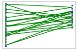
plt.scatter(x_test[:,0], y_test, color='blue')
plt.plot(x_test[:,0], y_pred, color='green', linewidth=3)
plt.xticks(())
plt.yticks(())
plt.show()
>>>

This chapter continues in the following part two.