Computer Vision, Search–Based Algorithms for Artificial Intelligence and Cognitive Science
Computer Vision is a class of Artificial Intelligence algorithms that works on images. Images can be in the form of static pictures or videos. Working through image–based data is complex, and therefore the internal packages like OpenCV that implement computer vision use various machine learning and search–based algorithms to implement computer vision. Along with using OpenCV, we will also take a look at these search–based algorithms and their implementations in the Computer Vision space.
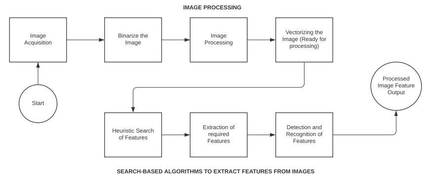
The only purpose of using search algorithms is to optimize the traversal through image space, since it is way more diversified than an array of integers. Image Processing on the other hand is a processing step in every Computer Vision algorithm. Let us now dive into how these search algorithms optimize processing of images and vectors.
Heuristic Search Algorithm
Most problems in AI are exponential in nature, meaning they have many possible solutions. It is hard to differentiate an incorrect solution from a correct one, and testing all solutions is costly. This is where Heuristic search comes in and eases the problem. Heuristic Search narrows down the options and eliminates the incorrect choices. A machine’s level of intelligence is often calculated based on the efficiency with which it performs heuristic search. So why do we need heuristics? The primary reason is speed. To produce a solution that is acceptable to the problem statement in a timeframe faster than any other algorithm. The solution here, need not be the best, but it should arguably be the fastest. Heuristic search allows us to reduce the exponential degree problem to a polynomial number. Where known algorithms do not work or uninformed searches take longer, since the environment size is large, heuristic search is the best bet.
Computer Vision and Heuristic Search: Images are stored in the form of vector matrices in a computer system. These vectors are numerical in nature since algorithms do not function on images and alphabets directly. Search algorithms are crucial in processing images since, even a small image has a large number of vectors to work on. Heuristic search helps in eliminating the vectors that are not important to the recognition algorithm. We will go through a few key search algorithms that are used in Computer Vision.
- Uninformed Search: This is also known as a blind control strategy, or blind search. The name is coined this way because the algorithm is presented with information only pertaining to the problem definition. There is no additional information provided. As a result, the algorithm needs to work on the entire input space to arrive at a solution. Depth First Search (DFS) and Breadth First Search (BFS) are a few key examples of uninformed search techniques.
- Informed Search: Heuristic Search is the informed search control strategy. The reason being these algorithms are given additional information that helps in speeding up their processing times. This information allows for generating preference between nodes of the input space. Best First Search and A* are a few examples.
- Constraint Satisfaction Problems (CSPs): Constraints literally stand for restrictions or limitations given to an algorithm. In terms of artificial intelligence, constraint satisfaction problems are given certain strict conditions under which they should perform. The primary objective of the algorithm is to not violate the given constraint and work within it. We will see the implementation of CSP in the section below.
# Solving Constraint Satisfaction Problems
# Majority of Computer Vision algorithms use CSP to build learning mechanisms, since the environment they are present in has numerous aspects that cannot be changed during analysis
# 1. Solving an algebraic equation: [a*2=b]
# The algorithm should return the values of a and b for a defined domain
# Install the necessary libraries and packages
pip install python–constraint
>>>
Downloading python–constraint–1.4.0.tar.bz2 (18 kB)
Building wheels for collected packages: python–constraint
  Building wheel for python–constraint (setup.py): started
  Building wheel for python–constraint (setup.py): finished with status 'done'
  Created wheel for python–constraint: filename=python_constraint–1.4.0–py2.py3–none–any.whl size=24086 sha256=a600eb3bc622b725c094af5097145dc850baf759c1b151d680b681de56020ebc
Successfully built python–constraint
Installing collected packages: python–constraint
Successfully installed python–constraint–1.4.0

# Import the constraint package using the following command:
from constraint import *
# Creating a new object Module for Problem()
object_prob = Problem()
# Now, we define the two variables with their range as 10 (The solution should come in first 10 numbers)
object_prob.addVariable('x', range(10))
object_prob.addVariable('y', range(10))
# Next, we define the required constraint
object_prob.addConstraint(lambda x, y: x * 2 == y)
# Creating the solution object using GetSolutions()
object_solution = object_prob.getSolutions()
print (object_solution)

>>> [{'x': 4, 'y': 8}, {'x': 3, 'y': 6}, {'x': 2, 'y': 4}, {'x': 1, 'y': 2}, {'x': 0, 'y': 0}]

# 2. We will now implement the Magic Square Problem.
# Magic Square: A square grid where numbers of a row, every column, and the diagonals, all add up to 'one' number –> Magic Constant
def function_magic_square(input_matrix):
    input_size = len(input_matrix[0])
    input_sum = []
    # Code for computing the vertical square
    for col_num in range(input_size):
        input_sum.append(sum(row_num[col_num] for row_num in input_matrix))
    # Code for computing the horizontal of the square matrix
    input_sum.extend([sum (lines) for lines in input_matrix])
    # Horizontal portion of the squares
    horizontal_result_l = 0
    for i in range(0, input_size):
        horizontal_result_l +=input_matrix[i][i]
    input_sum.append(horizontal_result_l)
    horizontal_result_r = 0
    for i in range(input_size–1, –1, –1):
        horizontal_result_r +=input_matrix[i][i]
    input_sum.append(horizontal_result_r)
    if len(set(input_sum))>1:
        return False
    return True

# Input the value of the matrix
print(function_magic_square([[4,2,1], [4,5,3], [3,2,9]]))

>>> False
# The output is false since the condition is not satisfied
# We will now try for a matrix that is a magic square
print(function_magic_square([[2,7,6],[9,5,1],[4,3,8]]))

>>> True
We discussed Heuristic Search in this code section. It is an important search technique used widely in Artificial Intelligence algorithms. This was the implementation of CSP in Python, but there are many other use cases of heuristic search.
Heuristics in Cognitive Science: Judgement and Decision Making
Cognitive computation systems are machines that generate goal–directed actions in response to the exposure they receive to the environment. An important characteristic of computing cognitive solutions is to process the local environment variables and connect them to the object in question. For instance, when running a face recognition system, an algorithm needs to understand the characteristics of the face (object in question) and successfully differentiate its features from the background of the image and other body parts (local environment). To process the uncertainties involved in this method, cognitive algorithms use heuristic search to eliminate distanced solutions. Apart from the search–based approach of looking at solving cognitive science problems, there are a few more techniques that help in improving the accuracy of performing computer vision. In the next section we will learn about the Minimax and Negamax algorithms and how they make computer vision more efficient.
Minimax and Negamax algorithms in Python
Apart from the search algorithms we discussed in the above section, we will now be looking at a few more algorithms that originate from a search–based technique and are used to speed up the execution of cognitive algorithms.
Minimax Algorithm: Combinational Search algorithms use heuristic search settings to speed up their execution. It is mostly used in multiplayer gaming titles. For instance, in multiplayer games that rely on one of the players tries to predict the move of their opponent and try to act based on that. This is called building a minimizing function. And in order to win this game, the player also tries to maximize their own function. Heuristic plays a significant role in the minimax strategy. Every node in the algorithm has its own heuristic function associated with it and this helps the pointer decide, moving to which node would benefit the solution the most.
Alpha–Beta Pruning: Minimax is combinational search, meaning it is an uninformed algorithm which seldom leads to exploring parts of the environment space that are not relevant. This wastes compute and storage resources. Alpha–Beta pruning is a strategy that helps the algorithm decide which parts of the space would yield relevant and faster results. It leaves the irrelevant part unexplored, hence saving resources. The goal of this technique is to avoid searching portions of the input that would not lead to a solution. Alpha in this case, is the maximum lower bound and Beta, stands for the minimum upper bound. These two values combined, restrict the movement of the pointer.
Negamax Algorithm: This is very similar to the Minimax algorithm but has a subtle and sophisticated implementation. In the minimax implementation, we define separate heuristic functions for the task of maximizing (increasing the chances of winning the game for player one) and minimizing (decreasing the chances of player two) outputs. In Negamax, we are able to work through both scenarios through the same heuristic function. This reduces total compute resource usage.
Genetic Algorithms for Optimization
Another computational group of search–based algorithms are the Genetic Algorithms (GAs). These function on the concept of gene selection and natural order of biological hierarchy. It is a subset of Evolutionary Computation, that is a much larger computational branch concentrating on gene–based algorithm building. John Holland from University of Michigan and his colleague David E. Goldberg are regarded as the pioneers of Evolutionary Computation and were responsible for building these set of optimization methods. GA(s) function by taking in a pool of possible solutions to a given problem. All the possibilities then undergo a set of recombination and mutations (similar to what we see in natural genetics). They then, produce children and this process is repeated for multiple generations. Every individual child that comes in a generation is assigned with a fitness value. This fitness value is based on the objective that the GA is trying to solve and the generations that yield higher fitness values are given a chance to mate and yield even fitter individuals. This continues until the stopping criterion (exit function) is reached. GAs is a great implementation of the Darwinian Theory of Survival of the Fittest. Genetic Algorithm structure is greatly randomized, and this nature of implementation gives great incentive for optimizing image processing algorithms. GAs performs a much better job in local search (given their attribute of working with historical data) then all other search algorithms and since images are part of a complex vector–based environment, this optimized way of searching allows for better processing and therefore faster execution of computer vision tasks. Following are the steps and stages that Genetic Algorithms work through. These steps are generally always sequential, and some might be repetitive based on the accuracy of the algorithm.
- Step 1: The input is read, and the first step is to randomly generate a possible solution, irrespective of its accuracy.
- Step 2: The initial solution is assigned a fitness value. This fitness value is kept as the comparable for all the future generation solutions.
- Step 3: Mutations and crossover operations are applied on the selected solution and these are then recombined. From this combination of solutions, the best fitness value is extracted.
- Step 4: The offspring of this newly generate best fitness solution is inserted to the population that initially gave us the first possible solution. Both these solutions are then crossed over and mutated. Their mutated output is checked for its fitness value.
- Step 5: If this new solution meets the stop condition, mutations are stopped and this is selected as the main solution, otherwise step 4 continues with more mutations and crossovers until the best fit solution based on the stop condition is met.
# https://www.linkedin.com/pulse/genetic-algorithm-implementation-python-ahmed-gad/
# This project is referenced from a package – PyGrad that was created by Ahmed Gad and has been open–sourced. Special mention and credits to his article and tutorial on GA – https://www.linkedin.com/pulse/genetic–algorithm–implementation–python–ahmed–gad/
# We need two additional packages to be installed to work with Genetic Algorithms
pip install pygad
import numpy
import functools
import operator
import matplotlib.pyplot
# Importing imageio to read the input image file
# More information about the pygad PyPI package here: https://pypi.org/project/pygad/
import imageio
import pygad
# Reading target image that has to be reproduced using GA
input_image = imageio.imread('test_flower.jpg')
input_image = numpy.asarray(input_image/255, dtype=numpy.float)
# We represent the image as a one–dimensional vector and return it
def image_to_vector(img_array):
return numpy.reshape(a=img_array, newshape=(functools.reduce(operator.mul, img_array.shape)))
# Convert the one–dimensional vector to an array
def vector_to_array(input_vector, shape):
# Checking whether reshaping is possible
if len(input_vector) != functools.reduce(operator.mul, shape):
raise ValueError("Reshaping failed")
return numpy.reshape(a=input_vector, newshape=shape)
# Target image after enconding. Value encoding is used.
image_encode = image_to_vector(input_image)
# We now calculate the fitness value for a solution from the population.
# The sum of absolute differences between individual genes values gives us the fitness value required.
def fitness_func(int_one, int_two):
fitness_value = numpy.sum(numpy.abs(image_encode–int_one))
# Negate the fitness value to turn it from decreasing to increasing
fitness_value = numpy.sum(image_encode) – fitness_value
return fitness_value
# Save the output of the run to a new image and enumerate the number of iterations taken
def callback_func(genetic_var):
if genetic_var.generations_completed % 500 == 0:
matplotlib.pyplot.imsave('Final_GA_Image_'+str(genetic_var.generations_completed)+'.png', vector_to_array(genetic_var.best_solution()[0], input_image.shape))
# Initiate the Genetic Algorithm class with the given parameters
genetic_var = pygad.GA(num_generations=20999,
num_parents_mating=12, # Number of Parent Solutions to consider
fitness_func=fitness_func, # Choosing which fitness function to use
init_range_low=0, # Lower scale entry point (Should be integer between 0–1)
init_range_high=1, # Higher scale exit point (Should be integer between 0–1)
sol_per_pop=22, # Number of populations to work through
num_genes=input_image.size, # Number of genes to use
mutation_by_replacement=True,
mutation_percent_genes=0.02, # % of genes from the population that need to be mutated
mutation_type="random", # Type of mutation
callback_generation=callback_func,
random_mutation_min_val=0,
random_mutation_max_val=1) # Mutation minimum and maximum values (range 0–1)
# Run the GA instance
genetic_var.run()
# Plot the GA run over time to see how image evolved
genetic_var.plot_result()
# We will now see some metrics for the best solution
int_one, result_fit, int_two = genetic_var.best_solution()
print("Selected Solution's Fitness Value = {result_fit}".format(result_fit=result_fit))
print("Iteration of the Selected Solution : {int_two}".format(int_two=int_two))
if genetic_var.best_solution_generation != –1:
print("Selected Solution was reached at the {best_solution_generation} generation.".format(best_solution_generation=genetic_var.best_solution_generation))
final_result = vector_to_array(int_one, input_image.shape)
matplotlib.pyplot.imshow(final_result)
matplotlib.pyplot.title("PyGAD & GARI for Reproducing Images")
matplotlib.pyplot.show()
>>>
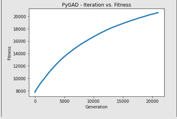 >>> Selected Solution's Fitness Value = 20551.29116769081
>>> Iteration of the Selected Solution : 0
>>> Selected Solution was reached at the 20998 generation.
>>>
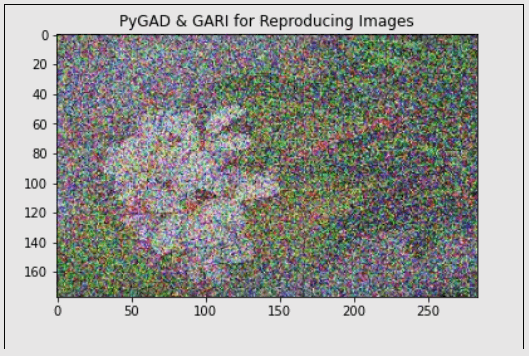 # This is the recreated image that the GA generated after 20998 mutations on the input. It is possible to get better solutions if the algorithm is allowed to run for even higher number of mutations and generations.
Image Processing in Python
Image Processing in simple terms is conversion of an image to its digital form and perform operations on it, generally to apply filters or extract features from the image. It can be seen as a form of signal dispensation where the input is generally in the form of images, which includes but is not limited to static images, videos, moving feature films, etc. Images are treated as two dimensional signals and converted to 2D vector arrays for the processing to take place. The purpose of Image Processing is to visualize the image input, clean any noise, seek for patterns, and lastly recognize features from the image. Image Processing is also termed Digital Image Processing in the computer vision domain. Image Processing is the pre–requisite feature engineering step of any computer vision problem. Below is a representation of how Image processing works. We will also look at a few key terms that all image processing pipelines use.
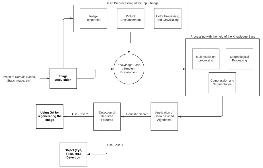
- Knowledge Base: Every problem needs its own domain to work. For instance, a video showing a cricket match would need an environment consisting of cricket equipment, grounds, pitches, and players. Similar to this, every image processing task also has its own knowledge base. Here, information about a problem domain is coded in the form of a database. The processing algorithm constantly operates with this database to check if the processes are going accurately.
- Morphological Processing: This is a shape–based processing of the image. Morphological processing pacts with operations and functions that are meant for extracting image components that would represent the image neatly in its dimensions (shape, size, and orientation).
- Image Segmentation: In any computer vision system, image segmentation is the process of portioning the image into smaller chunks of pixels or objects. The end goal here is to represent the image in a meaningful manner that would make analysis easier. It also assigns a label to every individual pixel which further helps machine learning and computer vision algorithms to work.
- Steps of Processing an Image: Image Processing is a multistep functionality that cannot be defined with a distinct set of occurring steps. These are dynamic and might have to be repeated from than once. Let us walk through the general pipeline of an image processing workflow:
- The first step is Image Acquisition that deals with ways of getting the image as input to the algorithm.
- Once the image input is captured, there are multiple preprocessing that is done on an image starting from scaling to cleaning it for noise to reformation of wavelets.
- Wavelets are the groundwork for signifying images in numerous degrees of resolution. Subdivision of images into smaller segments and regions for compression in the next step.
- Once the image is compressed it can be turned to 2D vectors and then search based algorithms we discussed above can work on the image vectors.
- The end goal of an image processing algorithm could be to detect a part of the image or regenerate the same image in different configurations.
Reading Images, Color Space Conversion and Edge Detection
OpenCV Functions for Image Processing
OpenCV is the most widely used library that allows image processing, including features for working with videos, human faces, etc. The underlying architecture of OpenCV uses Machine Learning algorithms to compute image processing tasks. Since working with images is much more complicated then working with numbers, OpenCV has an intense collection of algorithms that function with each other by breaking the recognition task into very small portions. Within these implementations are various search–based algorithms that we have seen earlier. To get started with OpenCV, we will go through the basic functions that allow reading, writing, and displaying images in Python:
- imread() function: This function is responsible for allowing user input in the form of images. It reads images from various file formats, including but not limited to PNG, JPEG, JPG and TIFF. It takes into argument, the file name, its path, and the extension.
- imshow() function: The ‘imshow’ function is used for seeing an image in Python on a new external window. The window that generates this output automatically fits to size of the image. This function too, supports numerous image formats like the read function. It takes into arguments the file name, path, and extension.
- imwrite() function: The write function is used to write binary data to an image file. Its general use–case is to convert the type of input file. The write function can save images in formats like PNG, JPEG, JPG, TIFF, etc. The desired extension is passed to its argument along with the desired file name.
Working with Images in Jupyter: When running a Jupyter instance of Python for using OpenCV, the imshow() function generates its output in a new window. This new image box uses the Python kernel that is running on Jupyter to process code. Since both executions work on the same kernel in an interactive shell, the kernel locks up when the program is executed. To solve this problem, we need to programmatically close the open windows, and this is where the
cv2.destroyAllWindows() functionality comes handy.
Let us now go through some code that will help us understand how to read image files in Python, convert images to grayscale and detect its edges using OpenCV. These procedures are the start of most image processing and computer vision algorithms.
# You can install this package with the help of the following command:
pip install opencv_python–X.X–cp36–cp36m–winX.whl
# The below command is specific to the Anaconda environment and can be run on its console for OpenCV installation.
conda install –c conda–forge opencv
import cv2
check_image = cv2.imread('test_flower.jpg')
cv2.imshow('Image of a Flower',check_image)
cv2.waitKey(0) #wait for any key
# Note: The function destroyallWindows() simply destroys all the windows we created.
cv2.destroyAllWindows()
>>> <function destroyAllWindows>
>>>
 # The “True” output here states that the format of the image is changed and it has been saved successfully
cv2.imwrite('image_flower.png',check_image)
>>> True
# The cvtColor() is a color conversion function that helps in changing the tone of the image’s color
image_new = cv2.cvtColor(check_image, cv2.COLOR_BGR2GRAY)
cv2.imshow('Grayscaled Flower',image_new)
cv2.waitKey(0)
cv2.destroyAllWindows()
>>>
 # Edge Detection in Images
# Now, use the Canny () function for detecting the edges of the already read image.
cv2.imwrite('Edge_Flowers.jpg', cv2.Canny(check_image, 200, 300))
# Display the Edge(d) Image
cv2.imshow('Edges of the Image', cv2.imread('Edge_Flowers.jpg'))
cv2.waitKey(0)
cv2.destroyAllWindows()
>>>
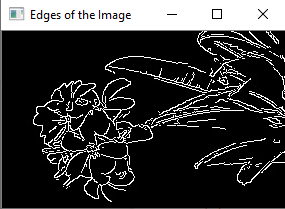 # We have now completed the Edge Detection, Gray scaling of images
Image classification into grayscaling and detection of edges is the first part of any processing algorithm. The reason being, grayscaled (black and white) images can be represeted as binary collection (0 – black, 1 – white) of vectors to the algorithm, which is easier to analyze. Similarly, edged images have a slightly lesser surface area, hence decreasing the overall size of the problem domain that speedens the analysis.
Face and Eye Detection
For working with something like a face or an eye, the algorithm breaks the detection task into numerous (6000 or more) smaller tasks that detect very small segments (collection of pixels) of the image and test whether it could be part of a face. OpenCV uses cascades for this part of the problem. A cascade is defined as a collection of waterfalls. Cascades are predefined battery of tests that the algorithm has to undergo in order to move to the next iteration. Cascades in OpenCV are XML files that contain data used by these algorithms to detect objects. Cascades are there for both human and non–human objects.
Face Detection
Face detection as the name suggests, is the branch of object detection that deals with identification of faces in the given image. The [“haarcascades/haarcascade_frontalcatface.xml”] cascade file is used for Face Detection. It occurs in the following steps:
- First the image is given as input to the program.
- Then the cascades are imported, and the face cascade class is initialized with the input image.
- Following conversion to grayscale, the detectMultiScale function is used to identify portions of the image that resemble a face. This function takes into input a grayscale image, a scale factor (some images might be closer to the camera and seem larger, therefore the image needs to be scaled to represent all possible objects in a specified scaled range), the minimum neighbors value defines object detected near the face and the min size argument gives a size of each window (individual small task)
- Finally, the algorithm forms a rectangle at every detected face.
import cv2
import numpy as np
# The path of differential variables we will be using
image_path = './Elon.jpg'
haarcasc_path = 'D:/Users/Anaconda/pkgs/libopencv–4.0.1–hbb9e17c_0/Library/etc/haarcascades/haarcascade_frontalcatface.xml'
# Create the haar cascade
face_cascade_class = cv2.CascadeClassifier(haarcasc_path)
# Read the image
test_image = cv2.imread(image_path)
gray_image = cv2.cvtColor(test_image, cv2.COLOR_BGR2GRAY)
# Detect faces in the image
checked_faces = face_cascade_class.detectMultiScale(
gray_image,
scaleFactor=1.2,
minNeighbors=3,
minSize=(10, 10)
)
# Draw a rectangle around the faces
for (x, y, w, h) in checked_faces:
cv2.rectangle(test_image, (x, y), (x+w, y+h), (0, 255, 0), 2)
cv2.imshow("Faces found", test_image)
cv2.waitKey(0)
cv2.destroyAllWindows()
cv2.imwrite('Face_EM_final.jpg',test_image)
>>> True
>>>
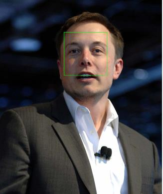 # We observe that the face border is seen in the output
This model seems to not have accurately identified the face. It can be improved by adjusting the scaling factor and changing the resolution of the image. Therefore, it is always considered a good practice to try the analysis with a combination of more than one set of configurations to see which one works perfectly.
Eye Detection
Detection of eyes is an after process of face recognition. The eye detection algorithm cannot function without segregating a face out of the image environment. The [“haarcascades/haarcascade_eye.xml”] cascade file is used to recognize eyes. All other steps are similar to what were executed in face detection.
import cv2
# The path of differential variables we will be using
image_path = './Eyes.jpg'
eye_haar_cascade = 'D:/Users/Anaconda/pkgs/libopencv–4.0.1–hbb9e17c_0/Library/etc/haarcascades/haarcascade_eye.xml'
eye_cascade_class = cv2.CascadeClassifier(eye_haar_cascade)
test_image = cv2.imread(image_path)
gray_image = cv2.cvtColor(test_image, cv2.COLOR_BGR2GRAY)
eyes = eye_cascade_class.detectMultiScale(gray_image, 1.2, 5)
for (ex,ey,ew,eh) in eyes:
test_image_eyes = cv2.rectangle(test_image,(ex,ey),(ex+ew, ey+eh),(0,255,0),2)
cv2.imshow("Eyes found", test_image_eyes)
cv2.waitKey(0)
cv2.destroyAllWindows()
cv2.imwrite('Eye_AB.jpg',test_image_eyes)
>>> True
>>>
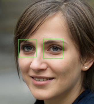 # We observe that the algorithm is able to segregate eyes from the input image
Similar to face detection, the eye detection algorithm can also be fine tuned to work better by changing the argument parameters in the function.
Coming up Next
With the completion of an introduction to Computer Vision, we have now traversed Cognitive Science in Artificial Intelligence. The key cognitive algorithms we worked on so far are NLP (Natural Language Processing), Speech Recognition and now Image Processing. In the coming chapters we will dive deeper into a case study involving cognitive science.
- Cognitive Science Case Study
- Understanding Facial Data
- Cognitive Modelling