Final Project and Python Implementation of AI

Project Initiation and Elicitation of Requirements

It is often called that the 21^st century is the birth of a digital age that will transform the way we interact with people and honestly, in the last few decades we have seen drastic changes in technology. Especially, communication methods have improved, and the entire globe is now connected on our fingertips. With the advent of Digital Information transformation, has come another revolution, namely, cyber fraud. Giving in to the ease of gathering and spreading information, the rise in counterfeit and misleading info has affected people and businesses across the world. With Artificial Intelligence, companies are now working towards making their data risk averse. In this chapter we will see a scenario of misleading news shared by websites on their webpages. We will use Machine Learning and Natural Language Processing to classify which news is real and which is fake. Finally, we will build a predictive model to predict any new news arrival and automatically classify it in the real or fake categories.

Understanding Misinformation and Forecasting Spam in News Reports

In recent years, we have seen an increase in the spread of misinformation, particularly on social media. Organizations, businesses, politicians, and individuals are all affected by this but at the same time are also involved in increasing this spread for their benefits. Media houses build an agenda of spreading fake news to manipulate people’s thoughts, for instance, during an election. This is an unethical practice and builds prejudice in the viewer’s thinking. Therefore, it leads us to question the integrity and authenticity of the news we see online today. Through this project, we will tackle this problem by studying patterns, websites, words, etc. that are most commonly used in creating fake news. We will also build a machine learning model to predict and subsequently classify a piece of information as fake or real.

Let us list the requirements that we will be looking to solve in this case study:

1. Understand factors that contribute to classification of news content.

2. Distinguish between fake and real news posted online on websites using Natural Language Processing.

3. Use cognitive modelling to understand words and facts presented in the news.

4. Build a classification model that predicts the category (real or fake) of the news by going through its contents.

5. Check the accuracy of the prediction model.

Cognitive Modelling

Cognitive Modelling is an area within computer science and specifically inside artificial intelligence that deals with the stimulation of a human’s problem-solving skills. This model’s goal is to simulate human thinking and predict behavior of humans. It is aimed at improving human-computer interaction. Human factors, neural networks, natural language processing, all these systems use cognitive modelling to build better programming results from machines.

Methodology of Processing Languages and Building a Classifier

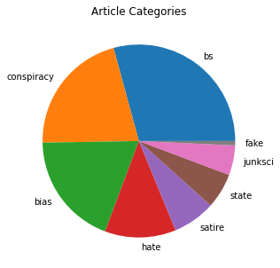
To solve the problem at hand, we will be working on the given methodology. The news collections data has a classified list of categories, namely, junk science, conspiracy, bias, satire, hate and this will help in building a category under which all the false news will fall under.

1. We will start the pre-processing with managing the text features of the dataset, in the following order:

   1. Removing and imputing all the NULL/Empty values.

   2. Next, we will transform categorical data into numerical data using the label encoders.

   3. All the text is moved to lowercase, for the NLP models to process efficiently.

   4. To work on tokenization, we will remove all the numbers from individual text sentences.

   5. Removing stop words, that would not contribute to the analysis, and then perform stemming.

2. We then perform lemmatization (with POS tagging) using the NLTK library.

3. In the feature engineering section of the analysis, the TF-IDF technique will be used.

4. Finally, this entire processed text will be put into the machine learning model as input for model’s training.

Project Implementation: Machine Learning and Text Processing

In this section we will be implementing the Fake News project. Let us go through the dataset.

About the Data: The data in this project is sourced from Kaggle and is available open source. It is derived from Meg Risdal’s data set present in the “Getting Real about Fake News” that contains numerous articles sourced from digital media to build a classifier. Finally, it is processed and kept in Kaggle’s News Classification database. We will explore the dataset in the code as well, but as a generalized structure, it contains news sources in the form of websites, labels showing whether the content is real or fake, and a column that presents news in a gist.

Predictive Modelling: Once the preprocessing portion of the analysis is over, the output we get will be a corpus of raw texts that do not contain any stop words. It will be stemmed and lemmatized in the NLTK processing and ready to be put input to the ML model. Before moving the text data into the machine learning model, we need to form a sparse matrix of TF-IDF values. To do this, we will be tokenizing the text, counting the tokens, and transforming these raw tokens into corresponding TF-IDF values. These steps ultimately help the Tfidf-Vectorizer (which we discussed in detail in the Natural Language Processing chapters). This vector will transform text to feature vectors that can then be used as numeric vectors to input into the estimators and classifiers.

New Libraries and Models Introduced:

1. Plotly: It is an open-sourced and a graphing library that builds interactive charts. It is a browser-based network that works with many languages like Python, R, MATLAB, and many others.

2. Cufflinks: It is a library that connects the data frame type from Pandas to Plotly for creating visualizations directly on Python. It creates interactive visualizations and is flexible since it binds with Pandas, which is crucial in Machine Learning.

3. Chart Studio: It is a library that builds on top of Plotly to run visualizations directly on the browser.

4. AdaBoost Classifier: The AdaBoost classifier is a machine learning training algorithm that works in iterations along with a base classifier (in this case we will be using a Decision Tree Classifier, with a maximum depth of 10 nodes). This inner classifier is to ensure precise predictions in case of any atypical observations. The algorithm runs on iterations and every iteration takes out the incorrect observations and gives those higher probability for getting classified in the incoming iteration.

5. Random Forest Classifier: A random forest is a meta classification mechanism that creates sub-samples of the input data and fits each sample with decision trees. It uses averaging to improve the predictions of the model and control over-fitting of data.

Now that we are ready with the prerequisites, we shall now begin the project and implement the logic explained above to Python code.

# We install the cufflinks and plotly libraries to build interactive visualizations and plots pip install cufflinks >>>


Requirement already satisfied: packaging in d:\users\anaconda\lib\site-packages (from bleach->nbconvert->notebook>=4.4.1->widgetsnbextension~=3.5.0->ipywidgets>=7.0.0->cufflinks) (20.4)

Requirement already satisfied: webencodings in d:\users\anaconda\lib\site-packages (from bleach->nbconvert->notebook>=4.4.1->widgetsnbextension~=3.5.0->ipywidgets>=7.0.0->cufflinks) (0.5.1)

Requirement already satisfied: pycparser in d:\users\anaconda\lib\site-packages (from cffi>=1.0.0->argon2-cffi->notebook>=4.4.1->widgetsnbextension~=3.5.0->ipywidgets>=7.0.0->cufflinks) (2.20)

Requirement already satisfied: pyparsing>=2.0.2 in d:\users\anaconda\lib\site-packages (from packaging->bleach->nbconvert->notebook>=4.4.1->widgetsnbextension~=3.5.0->ipywidgets>=7.0.0->cufflinks) (2.4.7)


pip install Plotly

>>>

Requirement already satisfied: retrying>=1.3.3 in d:\users\anaconda\lib\site-packages (from plotly) (1.3.3)

			Note: you may need to restart the kernel to use updated packages.


import pandas as pd

import matplotlib.pyplot as plt

import seaborn as sns

# We introduce a few new visualization libraries to build interactive plots

import cufflinks as cf

import plotly

import plotly.express as px



# importing the data into the notebook

news_df = pd.read_csv('news_articles.csv', encoding="latin", index_col=0)

news_df = news_df.dropna()

news_df.count()

>>>

published                  2045

title                      2045

text                       2045

language                   2045

site_url                   2045

main_img_url               2045

type                       2045

label                      2045

title_without_stopwords    2045

text_without_stopwords     2045

hasImage                   2045

dtype: int64



news_df.head(3)

>>>




 

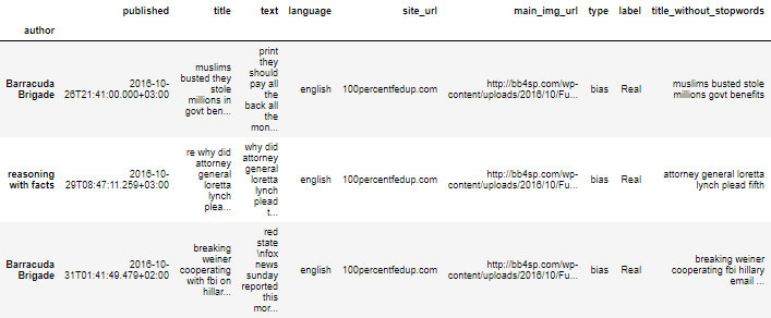# Let us now try to study the unique types of news categories present in the data set

news_df['type'].unique()

>>> array(['bias', 'conspiracy', 'fake', 'bs', 'satire', 'hate', 'junksci',

       'state'], dtype=object)



# Plot the different type of articles present in the dataset

news_df['type'].value_counts().plot.pie(figsize = (5,5))

plt.title('Article Categories')

plt.axis('off')

plt.show()

>>>





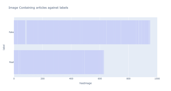
# Let us now look at the articles that contain images and the labels of their data

fig_img = px.bar(news_df, x='hasImage', y='label', title='Image Containing articles against labels')

fig_img.show()

>>>





# Let us take the list of websites that are producing articles used in the dataset

# We will later bifurcate this data and identify sites that give real vs fake news

news_df['site_url'].unique()

>>>

array(['100percentfedup.com', '21stcenturywire.com', 'abcnews.com.co',

       'abeldanger.net', 'abovetopsecret.com', 'activistpost.com',

       'addictinginfo.org', 'adobochronicles.com', 'ahtribune.com',

       'allnewspipeline.com', 'americannews.com',

       'americasfreedomfighters.com', 'amren.com', 'amtvmedia.com',

       'whatreallyhappened.com', 'whydontyoutrythis.com', 'wnd.com'],

      dtype=object)

….. <<Output Truncated>>

 

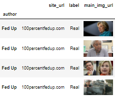
# From the above two outputs, let us now try to correlate images with their respective websites

def img2convert(imgpath):

    return '<img src="'+ imgpath + '" width="80">'

news_sources = news_df[['site_url','label','main_img_url']]

news_df_real = news_sources.loc[news_df['label']== 'Real'].iloc[6:10,:]

news_df_fake = news_sources.loc[news_df['label']== 'Fake'].head(6)



# Import the HTML library to work with HTML code embedded in the image column

from IPython.core.display import HTML

# We will now replace the HTML text with the actual image in the columns of the dataset

# Against Real News

HTML(news_df_real.to_html(formatters=dict(main_img_url=img2convert), escape=False))

>>>





# Against Fake News

HTML(news_df_fake.to_html(formatters=dict(main_img_url=img2convert), escape=False))

>>>





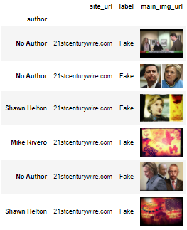# From the list of news websites we extracted, we now have the ones that have images, and ones with fake and real news

# Let us now label the real and fake news portions to further build our model

newstype_label = {'Real': 0, 'Fake': 1}

news_sources.label = [newstype_label[i] for i in news_sources.label]

real_value = []

fake_value = []

for i,row in news_sources.iterrows():

    val = row['site_url']

    if row['label'] == 0:

        real_value.append(val)

    elif row['label']== 1:

        fake_value.append(val)

 

# Import the Ordered Dictionary collection to segregate real and fake news websites

from collections import OrderedDict

# Real news publishing sites

unique_real_values = list(OrderedDict.fromkeys(real_value))

print(f"List of websites that generally publish real news:{unique_real_values}\n")

>>> List of websites that generally publish real news:['100percentfedup.com', 'addictinginfo.org', 'dailywire.com', 'davidduke.com', 'fromthetrenchesworldreport.com', 'frontpagemag.com', 'newstarget.com', 'politicususa.com', 'presstv.com', 'presstv.ir', 'prisonplanet.com', 'proudemocrat.com', 'redstatewatcher.com', 'returnofkings.com', 'washingtonsblog.com', 'westernjournalism.com', 'whydontyoutrythis.com', 'wnd.com']

 

# Fake news publishing sites

unique_fake_values = list(OrderedDict.fromkeys(fake_value))

print(f"List of websites that generally publish fake news:{unique_fake_values}\n")

>>> List of websites that generally publish fake news:['21stcenturywire.com', 'abcnews.com.co', 'abeldanger.net', 'abovetopsecret.com', 'activistpost.com', 'adobochronicles.com', 'ahtribune.com', 'allnewspipeline.com', 'americannews.com', 'americasfreedomfighters.com', 'amren.com', 'amtvmedia.com', 'awdnews.com', 'barenakedislam.com', ] …. <<Output Truncated>>

 

# The sites that publish both real and fake news

real_news_distinct = set(unique_real_values)

fake_news_distinct = set(unique_fake_values)

print(f"Websites that publish both real & fake news periodically:{real_news_distinct & fake_news_distinct}\n")

>>> Websites that publish both real & fake news periodically:{'davidduke.com', 'presstv.ir', 'westernjournalism.com', 'newstarget.com', 'fromthetrenchesworldreport.com', 'prisonplanet.com', 'washingtonsblog.com', 'frontpagemag.com', 'returnofkings.com'}



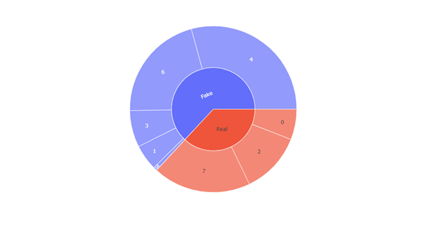
# We will now give every genre of news article their own label

genre_type = {'bias': 7, 'conspiracy': 6,'fake': 5,'bs': 4,'satire': 3, 'hate': 2,'junksci': 1, 'state': 0}

news_df.type = [genre_type[i] for i in news_df.type]



# Based on the genre of news, we now see which genre gives what portion of real and fake news

fig_genre = px.sunburst(news_df, path=['label', 'type'])

fig_genre.show()

>>>





# Chart Studio is another library that will help us build

pip install chart_studio

 

# Natural Language Processing

# Import the necessary NLP libraries

from sklearn.feature_extraction.text import CountVectorizer

from sklearn.feature_extraction.text import TfidfVectorizer

from pandas import DataFrame

# Cufflinks for visualization

cf.go_offline()

cf.set_config_file(offline=False, world_readable=True)

 

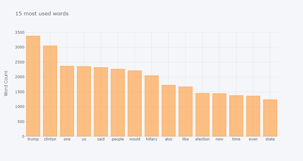
# Let us know use the NLP techniques practised in previous chapters to find out the most used words and phrases

# We first define a method to find the most occurring words in the input

def most_occuring_words(proc, n=None):

    vectorizer = CountVectorizer().fit(proc)

    bow = vectorizer.transform(proc)

    sum_of_words = bow.sum(axis=0)

    freq_of_word = [(word, sum_of_words[0, idx]) for word, idx in vectorizer.vocabulary_.items()]

    freq_of_word =sorted(freq_of_word, key = lambda x: x[1], reverse=True)

    return freq_of_word[:n]

 

used_words = most_occuring_words(news_df['text_without_stopwords'], 15)

words_df = DataFrame (used_words,columns=['word','count'])

words_df.groupby('word').sum()['count'].sort_values(ascending=False).iplot(

    kind='bar', yTitle='Word Count', title='15 most used words')

>>>





shuffled_news_df = news_df.sample(frac=1)

 

# Getting the features and labels ready for applying machine learning

b = shuffled_news_df.type

a = shuffled_news_df.loc[:,['site_url','text_without_stopwords']]

a['source'] = a["site_url"].astype(str) +" "+ a["text_without_stopwords"]

a = a.drop(['site_url','text_without_stopwords'],axis=1)

a = a.source

 

from sklearn.model_selection import train_test_split

from sklearn import metrics

from sklearn.ensemble import RandomForestClassifier, AdaBoostClassifier

from sklearn.neighbors import KNeighborsClassifier

from sklearn.tree import DecisionTreeClassifier

 

x_train,x_test,y_train,y_test = train_test_split(a,b,test_size=0.33)

input_vect_tfidf = TfidfVectorizer(stop_words = 'english')

vect_tfidf_train = input_vect_tfidf.fit_transform(x_train)

vect_tfidf_test = input_vect_tfidf.transform(x_test)

vectorized_df = pd.DataFrame(vect_tfidf_train.A, columns=input_vect_tfidf.get_feature_names())

 

# We will now use multiple Machine Learning algorithms to train and test their respective accuracies

# This will help in figuring out the best algorithm for the purpose

# ADA Boost Classifier

ada_boost_classifier = AdaBoostClassifier(DecisionTreeClassifier(max_depth=10),n_estimators=3)

ada_boost_classifier.fit(vect_tfidf_train, y_train)

ada_y_pred = ada_boost_classifier.predict(vect_tfidf_test)

ada_boost_accuracy = metrics.accuracy_score(y_test, ada_y_pred)

 

# Random Forest Classifier

random_forest_classifier = RandomForestClassifier(n_estimators=100)

random_forest_classifier.fit(vect_tfidf_train,y_train)

y_rand_pred = random_forest_classifier.predict(vect_tfidf_test)

random_forest_accuracy = metrics.accuracy_score(y_test, y_rand_pred)

 

# K-Nearest Neighbors Classification

knn_classifier = KNeighborsClassifier(n_neighbors=5)

knn_classifier.fit(vect_tfidf_train, y_train)

y_knn_pred = knn_classifier.predict(vect_tfidf_test)

knn_classifier_accuracy = metrics.accuracy_score(y_test, y_knn_pred)

 

# Comparision of individual accuracy scores

accuracy_scores = []

Used_ML_Models = ['ADA Boost Classifier','Random Forest Classifier', 'K-Nearest Neighbours']

accuracy_scores.append(ada_boost_accuracy)

accuracy_scores.append(random_forest_accuracy)

accuracy_scores.append(knn_classifier_accuracy)

 

score_comparisons = pd.DataFrame(Used_ML_Models, columns = ['Algorithms'])

score_comparisons['Accuracy on Training Data'] = accuracy_scores

score_comparisons

>>>

	Algorithms	Accuracy on Training Data
0	ADA Boost Classifier	0.957037
1	Random Forest Classifier	0.838519
2	K-Nearest Neighbours	0.515556

Our analysis shows that the ADA Boost Classifier outperforms the other classification algorithms and with this we conclude the Machine Learning Model. This is usually true for most of the NLP and text processing tasks because of the operation technique of this algorithm that continues to improve the incorrect classifications in every iteration.

Emotion Analysis, Conclusions and Learning

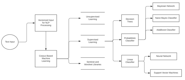
The above project showed us that analyzing text can also be used to understand its sentimental background and subsequently be utilized to predict if it is real or not. In this exercise we did not perform sentiment analysis as the data given to us was labelled. When dealing with raw text without labels, the approach would need to be that of analyzing the text’s sentiment and then trying to conclude whether or not it is true. Let us look at the below diagram to understand how emotion analysis can help in identifying the authenticity of content.



As we have seen earlier and also along this chapter, the concept of cognitive modelling can be used widely to help in analyses of various topics. The primary aim of artificial intelligence is to build machines that are closer to humans and those that can imitate human intellect responses. Cognitive Science is the approach, which is closest, a computer system can get to mimicking a human’s response. That’s the reason we have been concentrating deeply into these concepts for the last five chapters.

Coming Up Next

We have now covered all major concepts that revolve in the Artificial Intelligence using Python universe. Starting from programming basics in Python, implementing mathematical and statistical logic through code we learned the fundamentals of building math-based logic. Subsequently we moved to Machine Learning and its distinctive forms, before starting a deeper study of the human-AI connection in the form of Cognitive Modelling. In these chapters, we covered how processing natural languages, speech and facial data is making machines mimic human behavior and generate emotions. Artificial Intelligence has evolved dramatically and come very close to making machines enact human senses. The aim of this entire series was to establish grounds of implementing AI using Python. AI and Data are widely spread topics and the process of learning is never ending. It is therefore encouraged that you continue to explore, experiment, and build your intellect in all the topics covered here. As we end on this series, in the coming chapter we will walk through a theoretical section of how the present world is dealing with AI. Below are some key topics we will be covering:

1. The present AI and Data Science market

2. The rise of Cloud-Based implementation of AI

3. Continuing the learning process