Case Study 2 – Artificial Intelligence: Natural Language Processing

Revisiting Machine Learning from Case Study 1

During the first case study we built a machine learning pipeline that solved a prediction problem. We predicted house prices in the Ames region of Indiana based on multiple factors including, but not limited to land price, build quality, neighborhood, etc. There were a few key steps we took in building the machine learning pipeline. These steps form the basis of all machine learning problems.

1. Data Acquisition: All analysis needs data and data acquiring or collection is the process of getting that data to the model. Data can come from varied sources like web crawl, data warehouses, live streams of data like audio and video, etc. The acquired data can then be stored in the workspace in the form of Dataframes, that work seamlessly with Python’s analytics constructs.
2. Cleaning and Pre–processing: Raw data at most cases, contain information that may not help in the analysis and rather deprecate the predictions. Therefore, after data acquisition is complete, we perform some cleaning and pre–processing that includes steps like removing outliers, differentiating between features and labels, standardizing the features, deleting columns that will not contribute to analysis, imputing categorical variables, etc.
3. Exploratory Data Analysis: The EDA step is important at the beginning of the analysis since it reveals information about the data we are about to work on. EDA helps in understanding the data, finding patterns, categories and several statistical inferences like mean, median, standard deviation, and variance.
4. Building/Training the ML Model: Once all the data is ready for analysis and is standardized, we start building the machine learning model. The idea behind building a model is to provide it with plenty of data to learn. The algorithm uses this data to learn about patterns within the data and trains itself to work on unknown data of the same kind. Based on the problem and the desired solution there are a plenty of ML algorithms we can choose from, as we saw in the first case study.
5. Making Predictions: Finally, the output is the predictions that the ML model will make on unknown data. Once the algorithm is trained with data it understands how various points of information within the context are related to each other. During the prediction phase, the algorithm is fed with an input variable and its dependent value. The model ingests this input and predicts the desired output value.

We will be building a similar Machine Learning (ML) pipeline for analysis of language–based data in this case study. The only addition to this model will be steps of converting text to numeric and applying correct processing techniques to maintain the importance of individual words present in the textual input. Let us start working with NLP and integrate it to our Machine Learning workflow.

Addition of an NLP Layer to the Machine Learning Workflow

Within the machine learning pipeline, to include Natural Language Processing (NLP) we add a few steps during the Data Processing and cleaning phase. The training and testing algorithms still function the same way. The only logical change in the workflow is converting text into numeric data that the machine learning algorithm can work with. During this conversion, there are plenty of factors that need to be considered. For example, the number of times a word is occurring could help determine the topic being talked about.

Hybrid Approach to NLP and ML

Natural Languages are generally messy. Tones, interpretations, and meanings differ from person to person, and it is difficult to work a model that understands these concepts accurately. Therefore, Machine Learning alone cannot work an NLP solution. ML models are useful for recognizing the overall sentiment of a document or understand the entities present in the text. But they skirmish in extracting themes or matching sentiments to individual entities or themes. Therefore, in the Hybrid NLP approach we explain rules to the ML model. These rules are conventions that are followed in a language. These rules and patterns help the algorithm in relating classification more closely to human intuition.

The Bag of Words (BOW) Model in NLTK

Bag of Words (BoW) is an NLP model that is used in extraction of features from text and make it ready for modeling machine learning algorithms. This acts as an important step during extraction of features from input data. Once extracted, the features are then labelled with numeric data that ML algorithms work with, efficiently. The Bag of Words approach is simple as it does not regard weights to words. The logic separates every word in the sentence and paragraph into individual tokens. All these tokens are assigned a numerical value in a random order and these numbers do not have any order of precedence. The Count Vectorizer function within the sklearn Python package allows us to implement the BoW model. Let us know see a small application of this model.

# We will use the CountVectorizer from Scikit learn to convert the text into numeric vectors
from sklearn.feature_extraction.text import CountVectorizer
input_sent = ['Demonstration of the BoW NLTK model', 'This model builds numerical features for text input']
input_cv = CountVectorizer()
features_text = input_cv.fit_transform(input_sent).todense()
print(input_cv.vocabulary_)
>>> {'demonstration': 2, 'of': 9, 'the': 11, 'bow': 0, 'nltk': 7, 'model': 6, 'this': 12, 'builds': 1, 'numerical': 8, 'features': 3, 'for': 4, 'text': 10, 'input': 5}
# This allows us to build feature vectors that will successfully be used in Machine Learning algorithms.

Document Term Matrix: Since BoW does not regard for weights of words, there are scenarios where the predictions might go wrong. Document Term Matrix is a concept that contains the count of all occurring words within the document. With the help of this logic, all the words that BoW represents can be shown as a weighted sequence of numerous words. There is another algorithm (TF–IDF) that builds on top of BoW that uses weights of the words to form vectors.

TF–IDF (Term Frequency – Inverse Document Frequency): Every word has the same weight and importance in the Bag of Words model. But, in a real–world scenario, topics of discussion can be derived by understanding words that have been repeated in the context. The logic that TF–IDF follows is that those words which occur less in all the documents combined and occur many times in a single document have a higher contribution towards categorization of predictions. As the name suggests, TF–IDF is a combination of two interpretations (Term Frequency and Document Frequency). In simple words, it states that the classification value of a word increases if its term frequency (number of occurrences in a document) is higher and the inverse of document frequency (number of documents in which the word occurs) is higher. A typical use care of TF–IDF is Search Engine Optimization algorithms.

• TF = (Occurrence of a word in 1 document) / (Documents’ total words)
• IDF = Log ((Total number of documents) / (Count of documents that contain the Word))

TF–IDF using the Scikit–Learn Library The TfidfVectorizer class within Python’s Scikit–Learn library gives us a direct way of implementing the TF–IDF algorithm on text data. This class can be used to convert text features into TF–IDF feature vectors. Let us try to understand this algorithm using a Pseudo implementation of the model.

# Pseudo implementation of TF–IDF
import nltk
nltk.download("stopwords")
from nltk.corpus import stopwords
from sklearn.feature_extraction.text import TfidfVectorizer
input_vector = TfidfVectorizer (max_features=3000, min_df=6, max_df=0.75, stop_words=stopwords.words('english'))
output_features = input_vector.fit_transform(output_features).toarray()

In the code snippet above, let us try to understand the TfidfVectorizer function and all the parameters passed to it.

1. The ‘max_features’ definition is given as 3000, which means that the algorithm will only use the top 3000 most frequently occurring words from the document to create the Bag of Words (BoW). Less occurring words are generally not very useful for categorization.
2. The ‘max_df’ value denotes the percentage of documents where the word occurs. Here the algorithm will search for only those words that occur in 75% of the given documents. The reason is that words that are present in all the documents are also not very useful.
3. The ‘min_df’ value is for setting the cap of the minimum number of documents that should contain repeating words. In this case, the algorithm will consider words that have occurred in at least 6 documents to form the Bag of Words.

In the coming sections, we will start working on a scenario that requires Natural Language Processing (NLP). We will work on understanding emotions presented by humans through their written statements.

Case Study 2: Sentiment Analysis

Problem Statement: The input data set contains tweets sent out by users about six airlines within the United States. The aim is to categorize these tweets and messages into positive, neutral, and negative in sentiment. This will be done using a conventional supervised learning mechanism where the input training data set will be a determined from the tweets. With the training set, we will be building a model that creates categories.

Solution: The approach to this problem will involve a machine learning pipeline, like the one we used in Case Study 1. The initialization will start with importing the necessary libraries that are needed for this analysis. Exploratory data analysis is the next step where we will explore how the sections within the data are correlated and understand the input. We will next be adding a new step during the preprocessing where we will perform text processing. Since Machine Learning algorithms work effectively on numerical data, we will process the text input to numeric input (like what we saw above in the Bag of Words (BoW) model. Ultimately, once the preprocessing is complete, we will continue with the ML model and run it over for the entire dataset and understand its accuracy.

# Importing the necessary packages
import numpy as np 
import pandas as pd 
import re
import nltk 
import matplotlib.pyplot as plt
%matplotlib inline
# Data Source: https://raw.githubusercontent.com/kolaveridi/kaggle–Twitter–US–Airline–Sentiment–/master/Tweets.csv
import_data_url = "https://raw.githubusercontent.com/kolaveridi/kaggle–Twitter–US–Airline–Sentiment–/master/Tweets.csv"
sentiment_tweets = pd.read_csv(import_data_url)

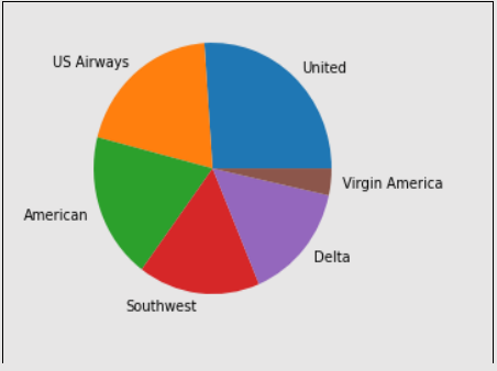
# Running EDA on the input data set to understand it better. Distribution of tweets based on the airlines
sentiment_tweets.airline.value_counts().plot(kind='pie', label='')
>>> <AxesSubplot:>
 


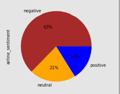
# Distinguish between the type of sentiments shown by users
sentiment_tweets.airline_sentiment.value_counts().plot(kind='pie', autopct='%1.0f%%', colors=["brown", "orange", "blue"])
>>> <AxesSubplot:ylabel='airline_sentiment'>



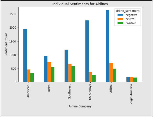
airline_grouped_sentiment = sentiment_tweets.groupby(['airline', 'airline_sentiment']).airline_sentiment.count().unstack()
airline_grouped_sentiment.plot(figsize=(8,5), kind='bar', title='Individual Sentiments for Airlines', xlabel='Airline Company', ylabel='Sentiment Count')
>>> <AxesSubplot:title={'center':'Individual Sentiments for Airlines'}, xlabel='Airline Company', ylabel='Sentiment Count'>



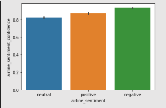
import seaborn as sns
sns.barplot(x='airline_sentiment', y='airline_sentiment_confidence' , data=sentiment_tweets)
>>> <AxesSubplot:xlabel='airline_sentiment', ylabel='airline_sentiment_confidence'>



# Cleaning of data: Since these tweets might contain punctuation marks and other non–relevant characters, we will process those and remove them from the model
# Let us also divide the feature and label sets for this data
feature_set = sentiment_tweets.iloc[:, 10].values
label_set = sentiment_tweets.iloc[:, 1].values
cleaned_feature_set = list()
for input_phrase in range(0, len(feature_set)):
    # 1. Removing all the special characters (*,etc.) and single characters (a,an,etc.)
    clean_feature = re.sub(r'\W', ' ', str(feature_set[input_phrase]))
    clean_feature= re.sub(r'\s+[a–zA–Z]\s+', ' ', clean_feature)
    clean_feature = re.sub(r'\^[a–zA–Z]\s+', ' ', clean_feature) 
    # 2. Convert the entire phrase to lower cases
    clean_feature = clean_feature.lower()
    cleaned_feature_set.append(clean_feature)

# Changing the text to a numerical form: All machine learning and statistical models use mathematics and numbers to compute data. Since the input here is textual, we will use the TF–IDF scheme to process words.
# Import the necessary packages
from nltk.corpus import stopwords
from sklearn.feature_extraction.text import TfidfVectorizer
input_vector = TfidfVectorizer (max_features=3000, min_df=6, max_df=0.8, stop_words=stopwords.words('english'))
cleaned_feature_set = input_vector.fit_transform(cleaned_feature_set).toarray()

# Let us now use the Train, Test, Split function to divide this data into training and testing sets. We will use the training set to train the model and find the best suitable model for this prediction and then run that model on the test data to finalize the prediction score
from sklearn.model_selection import train_test_split
X_train, X_test, y_train, y_test = train_test_split(cleaned_feature_set, label_set, test_size=0.33, random_state=42)
from sklearn.ensemble import RandomForestClassifier
from sklearn.linear_model import LogisticRegression
from sklearn.svm import SVC
from sklearn.neighbors import KNeighborsClassifier
from sklearn.metrics import accuracy_score
# Random Forest Classification
rf_classifier = RandomForestClassifier(n_estimators=200, random_state=42)
rf_classifier.fit(X_train, y_train)
rf_classifier_score = rf_classifier.score(X_train, y_train)
# Support Vector Machine Linear Classification
svc_classifier = SVC(kernel='linear')
svc_classifier.fit(X_train, y_train)
svc_classifier_score = svc_classifier.score(X_train, y_train)
# Logistic Regression
lr_classifier = LogisticRegression(random_state=0, solver='lbfgs', multi_class='ovr').fit(X_train, y_train)
lr_classifier_score = lr_classifier.score(X_train, y_train)
# K–Nearest Neighbors Classification
knn_classifier = KNeighborsClassifier(n_neighbors=5)
knn_classifier.fit(X_train, y_train)
knn_classifier_score = knn_classifier.score(X_train, y_train)

# Comparision of individual accuracy scores
accuracy_scores = []
Used_ML_Models = ['Random Forest Classification','Support Vector Machine Classification','Logistic Regression',
                   'KNN Classification']
accuracy_scores.append(rf_classifier_score)
accuracy_scores.append(svc_classifier_score)
accuracy_scores.append(lr_classifier_score)
accuracy_scores.append(knn_classifier_score)
score_comparisons = pd.DataFrame(Used_ML_Models, columns = ['Classifiers'])
score_comparisons['Accuracy on Training Data'] = accuracy_scores
score_comparisons
>>> 
                Classifiers	                                              Accuracy on Training Data
0	Random Forest Classification	              0.992965
1	Support Vector Machine Classification         0.859808
2	Logistic Regression	                              0.820759
3	KNN Classification	                              0.797308
# We see that the Random Forest Classifier performs the best
# Final prediction using the best–case algorithm from the above table
final_pred = rf_classifier.predict(X_test)
# Accuracy score of the final prediction
print(accuracy_score(y_test, final_pred))
>>> 0.7667632450331126
 

We observe that the prediction score on test data is not as good as it was on the training data. But, since Random Forest was our best resulting algorithm, to improve this score, we could build the model with better rules. The pre–processing phase that adds additional rules to be followed by the algorithm adds a lot of meaning to the analysis. Building better rules can always increase accuracy since concepts of grammar, parts of speech and other etymologies that we use in everyday languages is not known to the NLP model. We give the model these rules during the processing phase of model creation. With this we conclude the Sentiment Analysis project and move to general use cases of Natural Language Processing.

Natural Language Processing and its Use Cases

NLP is an artificial intelligence notion that recognizes and understands languages used by humans, both in the spoken and written forms. There are several use cases of NLP that are used across industries and businesses. Let us discuss a few key use–cases powered by NLP.

• Epidemiological Investigation: Processing of natural languages is used to read through medical records, diagnosis, and reference materials to predict anomalies in symptoms. For example, Alibaba used this technique along with StructBert NLP model to understand the variations of flu–based diseases in their fight for COVID–19 in cities of China.
• Security Authentication: By studying user information, NLP is used to generate advanced questions for securing a user’s system. The entity recognition model is used to extract relevant answers from a user’s security questionnaire. Neural networks are then used to generate more advanced questions for securing the user’s entity.
• Brand Awareness and Market Research: Sentiment analysis is extensively used in market research. When a user purchases a product, they are asked for their review of the product. The analysis of these reviews helps understand features of the product and build on the weak elements. It also helps in understanding what brands and products people prefer.
• Chat–Bots: Automated chat bots are frequently used in various websites to help users in their queries by talking to them. Chat bots are built on NLP and use conversational models to respond to users with relevant answers to their questions.
• Gathering Intelligence in Real–Time, for Financial Stocks: The stock market is highly sensitive to world news and organizational changes. Understanding these changes are key in making stock decisions. Therefore, many companies use NLP to work through news updates and organizations’ board updates to predict the trend of their stocks in the future.
• Defense Organizations: Defense organizations in many countries including the United States (Department of Defense) work with companies like Facebook, Google and Microsoft that hold a lot publicly available information to build a deep learning predictive network that reads conversation trends to envisage any security breaches in the near future.

Categorization of text is an important feature that majority of algorithms use. NLP can also be used for the same, and we will see this in the implementation below where we try to categorize the main topic of the input sentences.

# Import the necessary packages
from sklearn.datasets import fetch_20newsgroups
from sklearn.naive_bayes import MultinomialNB
from sklearn.feature_extraction.text import TfidfTransformer
from sklearn.feature_extraction.text import CountVectorizer

# Creating a dictionary based on the input data package to classify the results
dict_cat = {'talk.religion.misc': 'Religious Content', 'rec.autos': 'Automobile and Transport','rec.sport.hockey':'Sport: Hockey','sci.electronics':'Content: Electronics', 'sci.space': 'Content: Space'}
data_train = fetch_20newsgroups(subset='train', categories = dict_cat.keys(), shuffle=True, random_state=3)
cv_vector = CountVectorizer()
data_train_fit = cv_vector.fit_transform(data_train.data)
print("\nTraining Data Dimensions:", data_train_fit.shape)
>>> Training Data Dimensions: (2755, 39297)

# Import the TF–IDF Transformer
tfidf_transformer = TfidfTransformer()
train_tfidf_transformer = tfidf_transformer.fit_transform(data_train_fit)
# Input data for running sample sentences
sample_input_data = [
'The Apollo Series were a bunch of space shuttles',
'Islamism, Hinduism, Christianity, Sikhism are all major religions of the world',
'It is a necessity to drive safely',
'Gloves are made of rubber',
'Gadgets like TV, Refrigerator and Grinders, all use electricity'
]
# Using the Multinomial Naïve Bayes’ classification mechanism with TF–IDF
input_classifier = MultinomialNB().fit(train_tfidf_transformer, data_train.target)
input_cv = cv_vector.transform(sample_input_data)
tfidf_input = tfidf_transformer.transform(input_cv)
predictions_sample = input_classifier.predict(tfidf_input)
for inp, cat in zip(sample_input_data, predictions_sample):
    print('\nInput Data:', inp, '\n Category:', \
        dict_cat[data_train.target_names[cat]])
>>> 
Input Data: The Apollo Series were a bunch of space shuttles 
 Category: Content: Space

Input Data: Islamism, Hinduism, Christianity, Sikhism are all major religions of the world 
 Category: Religious Content

Input Data: It is a necessity to drive safely 
 Category: Automobile and Transport

Input Data: Gloves are made of rubber 
 Category: Automobile and Transport

Input Data: Gadgets like TV, Refrigerator and Grinders, all use electricity 
 Category: Content: Electronics
 

These are the results of the categorization for the input sentence and with this we conclude the analysis of Natural Languages.

Coming up Next

Through the last two chapters we worked on problems that span around Natural Language Processing (NLP). We learned how NLP is gaining popularity among Artificial Intelligence algorithms. There are several problems that NLP can solve, and we have seen the steps we follow to build the language processing pipeline. In the next few chapters, we will dive deeper into Cognitive Artificial Intelligence and work on concepts of Computer Vision and Speech based analysis of data. All the upcoming chapters and models in AI, follow a similar structure and workflow that we have discussed in the last two case studies. These are few key concepts coming up next:

1. Working with Speech based data
2. Spoken words and Audio Signals
3. Computer Vision using Python